In the previous post you created a pivot table in Excel. Now your manager wants you to do it in Tableau. How would you do it?
The process is very similar.
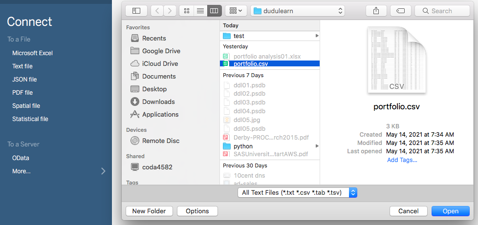
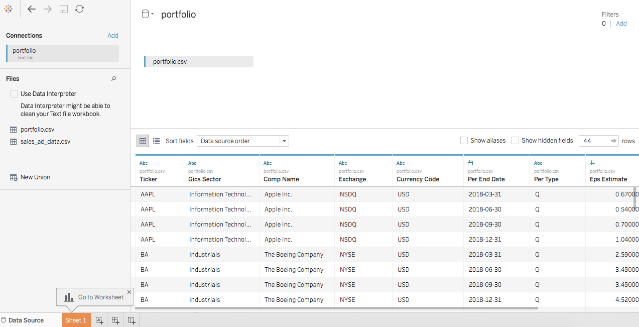
First, let’s import the data. Assume the data comes as csv file.
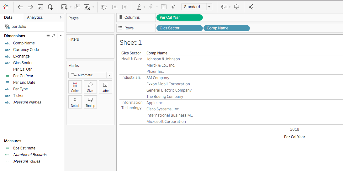
Now click Sheet1. Drag Gics Sector and Comp Name to the Rows Shelf, and Per Cal Year to the Columns Shelf.
Note the color of Per Cal Year is green. This is because Tableau treats the time dimension as continuous by default.
Since we are displaying a pivot table instead of a chart, let’s change Per Cal Year to discrete.
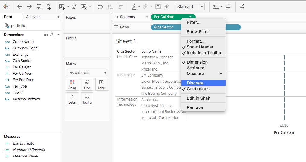
Now you will see the color of Per Cal Year changed to blue.
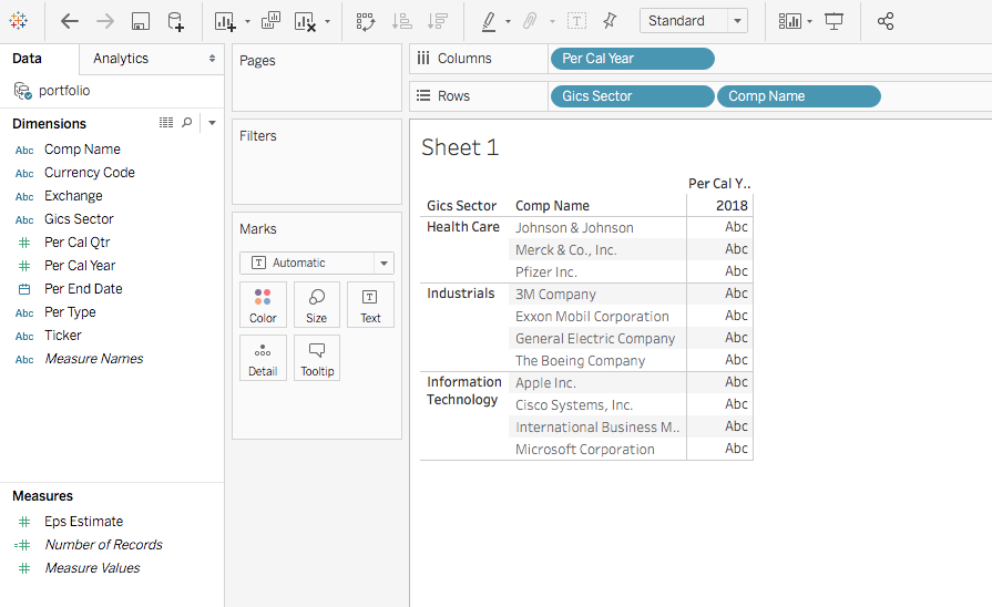
Now double click Eps Estimate under Measures (or drag Eps Estimate to the Abc area of the pivot table.
You will see the Eps Estimate is displayed as SUM by default.
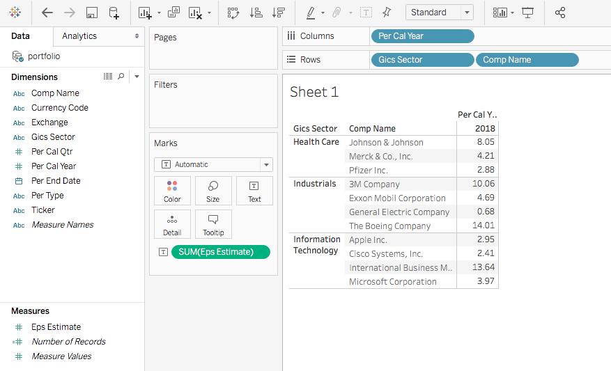
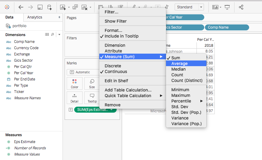
Right click SUM(Eps Estimate), go to Measure (Sum) and tick Average.
The eps_estimate is showing as average now. Let’s format the number to two digits.
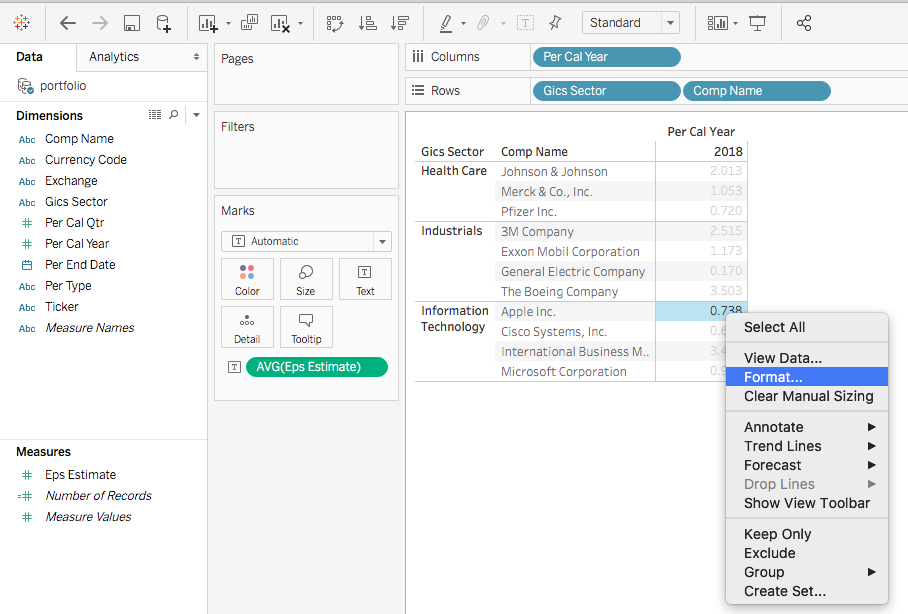
Right click any value cell, click to Format.
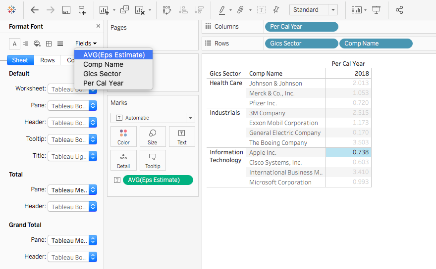
Click the Fields dropdown, select AVG(Eps Estimate).
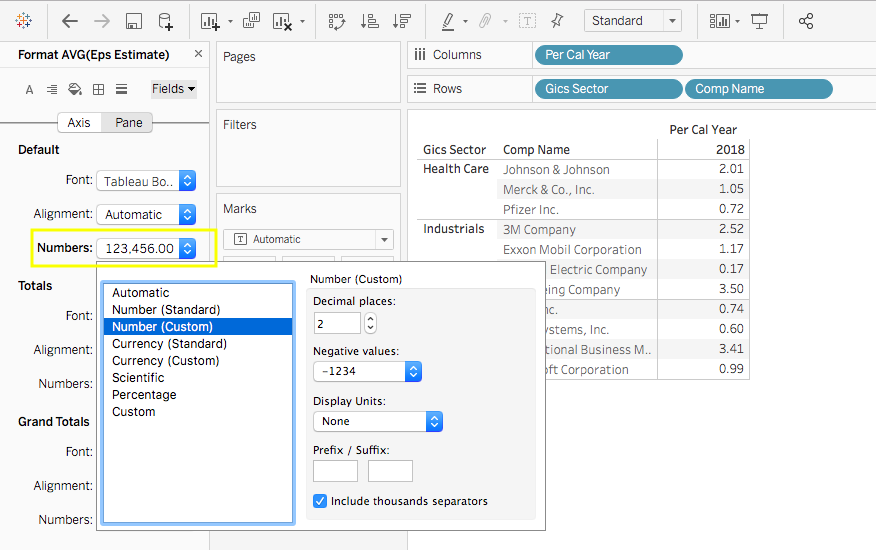
Select Numbers dropdown in the Default area, and pick Number (Custom).
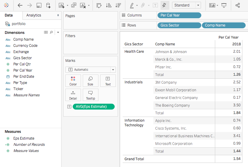
As a result, the average eps_estimate will be displayed as 2 digits.
Now let’s show average eps_estimate of each industry sector. Go to Analysis -> Totals -> Add All Subtotals.
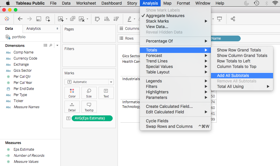
Let’s also show average eps_estimate of the entire portfolio. Go to Analysis -> Totals -> Show Column Grand Totals.
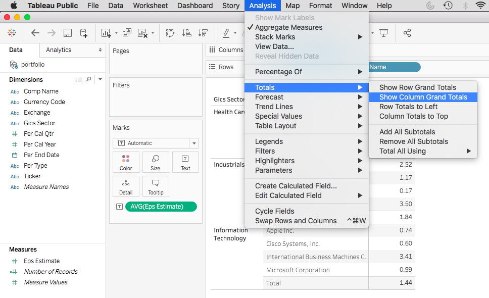
Now you have your pivot table ready to go!