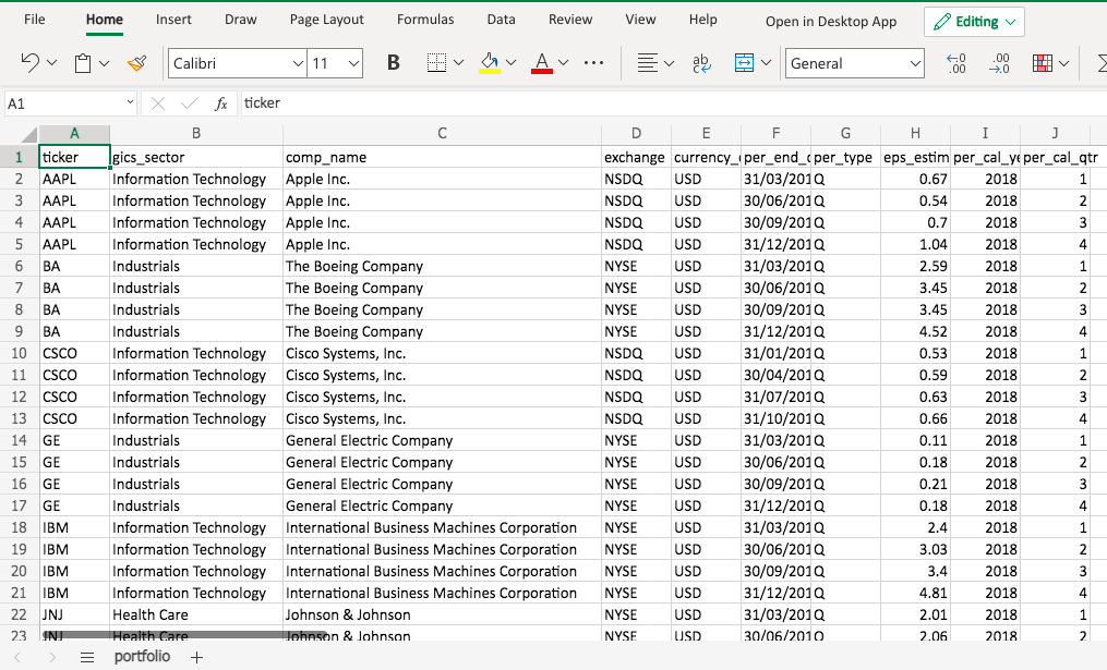
You are a portfolio analyst at an Investment company. Your manager gave you a dataset and asked you to conduct a few tasks to answer a few questions. How would you handle it?
- Provide a summary of the portfolio. What sectors does the portfolio cover?
- For a specific fiscal year, what is the average EPS (earnings per share) estimate for each stock?
- What is the average EPS estimate for each industry sector?
Pivot table enables analyst to quickly summarize data.
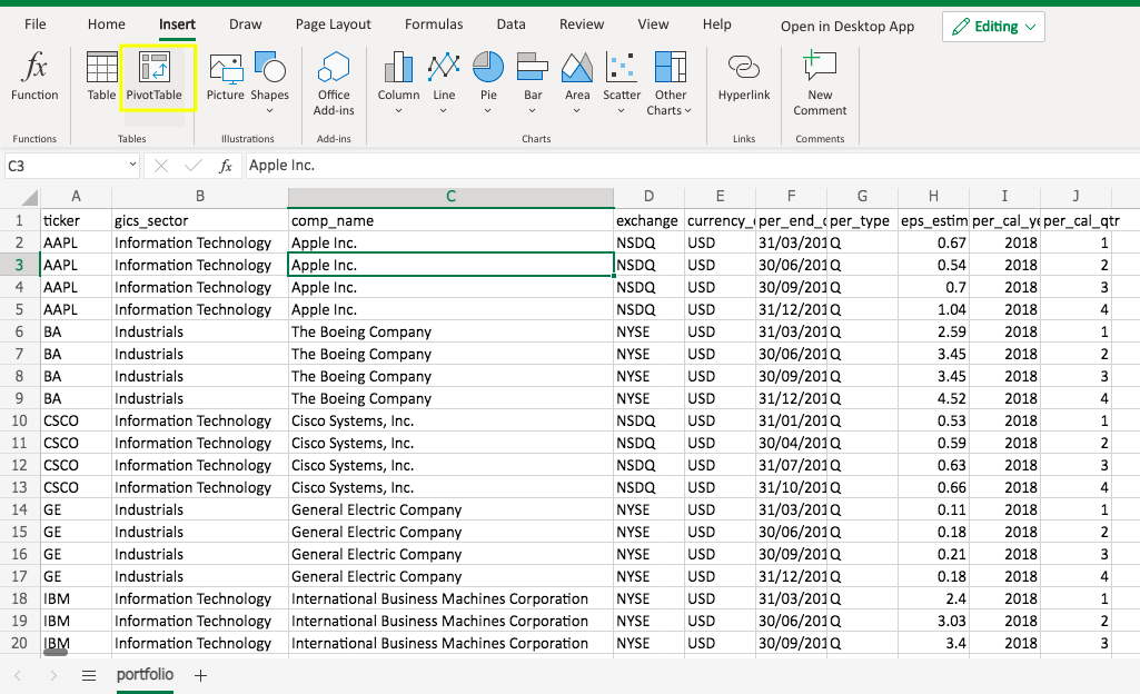
To create a pivot table, click any cell in the data source range. Go to Insert -> Pivot Table.
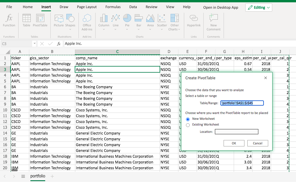
A pop-up will give you the default data source range to edit and ask you whether to create the pivot table on a new sheet by default. Simply click OK.
Then you will see a new sheet created, with a blank pivot table and the pivot table field list.
Now drag the gics_sector and comp_name to the ROWS area, per_cal_year to the COLUMNS area, and eps_estimate to the VALUES area. You will get an initial version of pivot table.
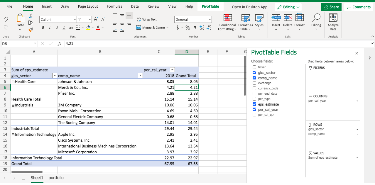
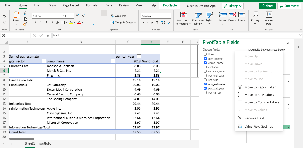
Note in the VALUES area, eps_estimate becomes Sum of eps_estimate. That’s the default function when we aggregate values. Let’s modify the function by clicking the triangle dropdown.
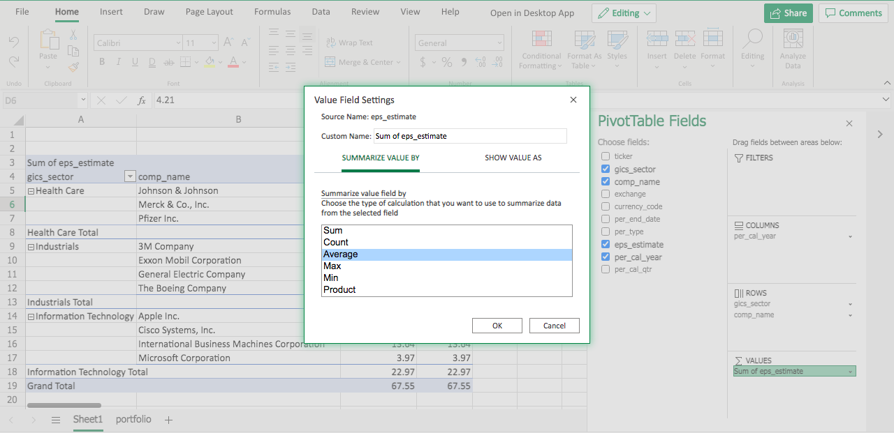
Under SUMMARIZE VALUE BY, select Average, and click OK.
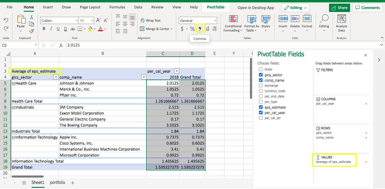
Then you will see the eps_estimate is displayed as the Average now. Note the number format isn’t standardized. To adjust it, one quick way is to select the value cells range, and click the comma sign.
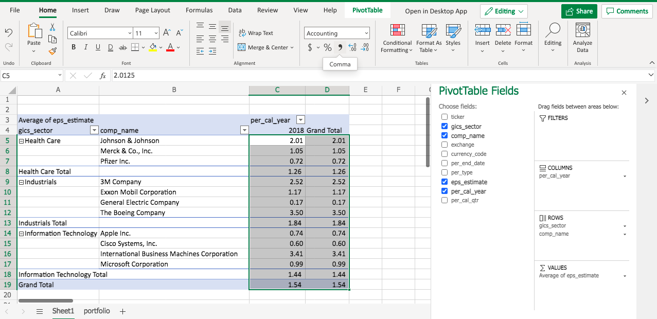
As a result, the average eps_estimate will be displayed as 2 digits.
Now you pretty much have your pivot table ready, and you should be able to answer your manager’s questions.
